How to actually optimize neural network training in PyTorch
The aim of this blog post is to speed-run the best quick tips and tricks for optimizing the latency, memory footprint, and performance of model training in PyTorch.
Table of contents
Profiling
The first thing you should always do when training neural networks on a GPU is to check that you are close to 100% GPU utilisation. If you are not then you are wasting valuable GPU time letting it sit idle and can make easy gains on almost any project by improving this. To check this once you can ssh onto your GPU and run nvidia-smi.
To visualize GPU memory usage in depth, you can use:
torch.cuda.memory._record_memory_history(max_entries=100_000)

# We will profile 3 training steps:
for step, (input, target) in enumerate(train_loader):
	output = model(input)
	loss = loss.backward()
	optimizer.step()
	optimiezer.zero_grad()

	if step == 2:
		torch.cuda.memory._dump_snapshot(filename="snapshot.pickle")
		torch.cuda.memory._record_memory_history(enabled=None)
		break
Then take your snapshot.pickle file and drop it here: https://docs.pytorch.org/memory_viz.
This will give you a plot that looks something like:
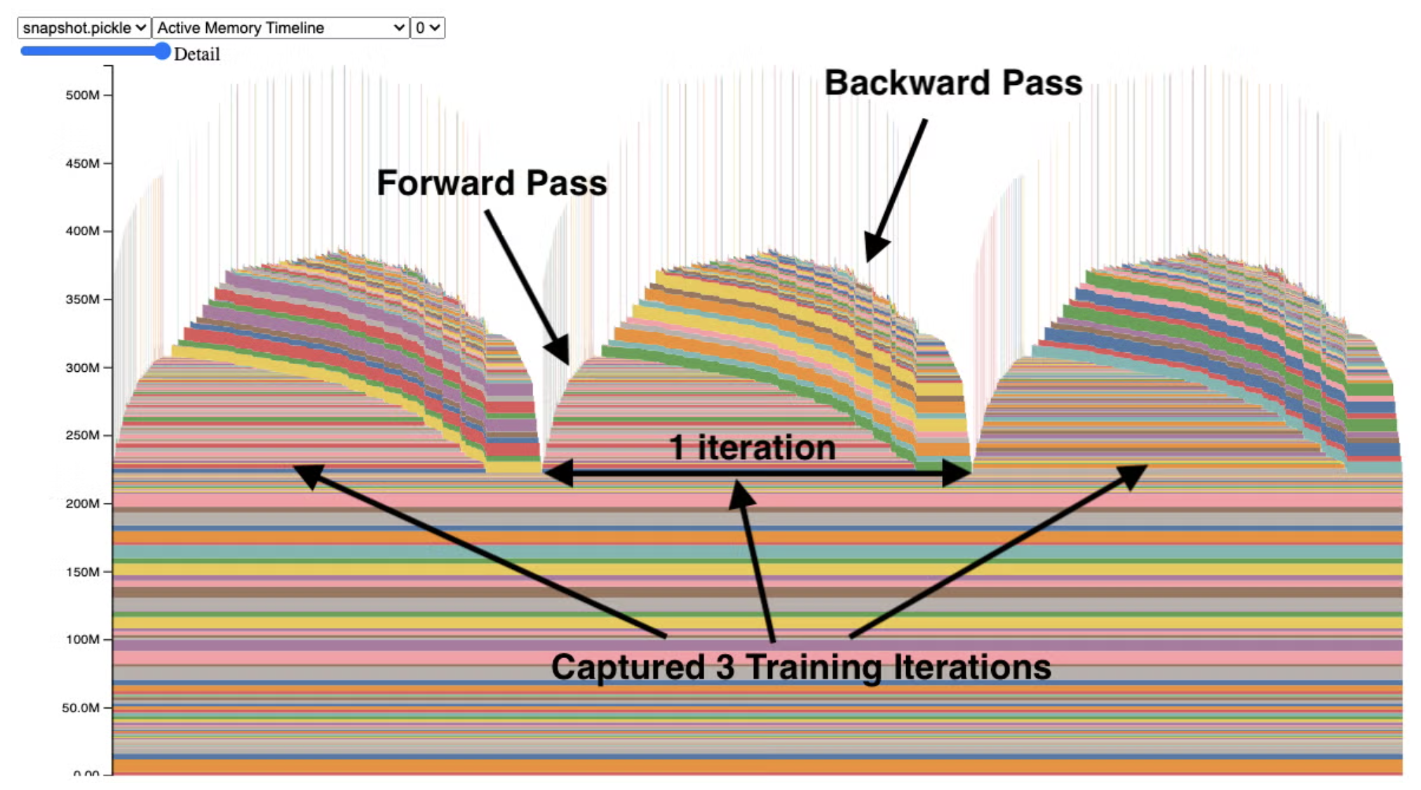
Each component is some activity on the GPU; hover over them for a breakdown.
Memory and latency
torch.compile
You can massively reduce the latency and memory footprint of your model using torch.compile. This comes basically for free and takes just one line to implement:
model = torch.compile(model, backend="inductor")
https://docs.pytorch.org/tutorials/intermediate/torch_compile_tutorial.html
Automatic mixed precision training
The default precision of weights, activations, and gradients in PyTorch is float32. However, we can substantially reduce the latency and memory footprint of the model by reducing this precision (e.g., using float16). This is optimal for operations like linear layers and convolutions, but other operations like reductions require the dynamic range of float32. PyTorch’s amp package handles all of this for us automatically.
One problem is that gradients can be so small that they cannot be represented in low precision. This is called underflow and we can fix it by scaling the loss by a large factor before the backward pass, then unscaling the gradients before the optimizer step. This can be done with PyTorch’s GradScaler.
from torch.amp import autocast, GradScaler
from torch.optim import SGD

# Assume we have defined Net (model), epochs (number of epochs), and data.

# Creates model and optimizer in default precision
model = Net().cuda()
optimizer = SGD(model.parameters(), ...)

# Creates a GradScaler once at the beginning of training.
scaler = GradScaler()

for epoch in epochs:
    for input, target in data:
        optimizer.zero_grad()

        # Runs the forward pass with autocasting.
        with autocast(device_type='cuda', dtype=torch.float16):
            output = model(input)
            loss = loss_fn(output, target)

        # Scales loss.  Calls backward() on scaled loss to create scaled gradients.
        # Backward passes under autocast are not recommended.
        # Backward ops run in the same dtype autocast chose for corresponding forward ops.
        scaler.scale(loss).backward()

        # scaler.step() first unscales the gradients of the optimizer's assigned params.
        # If these gradients do not contain infs or NaNs, optimizer.step() is then called,
        # otherwise, optimizer.step() is skipped.
        scaler.step(optimizer)

        # Updates the scale for next iteration.
        scaler.update()
Gradient accumulation
If you want to increase your batch size but are bottlenecked by GPU memory, use gradient accumulation to sum gradients over multiple steps before updating the weights. This increases your “effective” batch size by a factor of grad_acc_steps.
grad_acc_steps = 5 # effective batch size increases x5

for i, (input, target) in enumerate(train_loader):

	out = model(input)
	loss = loss_fn(out, target)
	loss.backward() # accumulate gradients

	if step % grad_acc_steps == 0:
		optimizer.step()
		optimizer.zero_grad()
Gradient checkpointing
By default, PyTorch stores all intermediate activations during the forward pass to use in backpropagation, which takes up lots of memory. With gradient checkpointing, we can discard these activations and recompute them on-the-fly during the backward pass. This trades extra compute for less memory usage, enabling you to train much larger models or use bigger batch sizes.
import torch
import torch.nn as nn
from torch.utils.checkpoint import checkpoint

class DeepModel(nn.Module):
    def __init__(self, use_checkpointing=False):
        super().__init__()
        self.use_checkpointing = use_checkpointing

        # Define multiple transformer-like blocks
        self.blocks = nn.ModuleList([
            nn.TransformerEncoderLayer(d_model=512, nhead=8)
            for _ in range(12)
        ])

    def forward(self, x):
        for block in self.blocks:
            if self.use_checkpointing:
                # Trade compute for memory: don't store intermediate activations
                x = checkpoint(block, x, use_reentrant=False)
            else:
                # Standard forward: stores all activations for backward pass
                x = block(x)
        return x

model = DeepModel(use_checkpointing=True)

# Dummy input: (sequence_length, batch_size, d_model)
x = torch.randn(100, 32, 512, requires_grad=True)

output = model(x)
loss = output.sum()
loss.backward()  # Recomputes activations during backward pass

print("Gradient checkpointing saves ~8-10x memory for deep models!")
Performance and stability
Optimal batch size
In most domains of generative modelling (language, audio, imaging. etc.), it is usually preferable to use large batch sizes. This is for time-efficiency (we need fewer training steps) and to avoid excessive noise in the gradients. However, there exists a ‘critical’ batch size beyond which your gradients have such little noise that adding extra examples just takes up extra compute with no added benefit.
This is explored in OpenAI’s “An Empirical Model of Large-Batch Training”, which proposes a measurable statistic to predict the maximum effective batch size.
When experimenting with batch size, it is generally advised to adjust your learning rate accordingly. With large batch sizes, your gradients are more accurate and so you can afford to take a larger step, but small batches lead to noisy gradients and it is better to take smaller steps. It is common to scale learning rate linearly with either the batch size or the square root of the batch size.
Gradient clipping
Clipping your gradients will avoid unstable training by prevent excessively large updates:
for step, (input, target) in enumerate(train_loader):
	output = model(input)
	loss = loss_fn(output, target)
	loss.backward()

	torch.nn.utils.clip_grad_norm_(model.parameters(), max_norm=5)
Exponential moving average
An exponential moving average (EMA) of your model often performs better than the base model. There is a decent guide here.
from copy import deepcopy

# start with some model
model = MyTransformer(device="cuda")
eta = 0.02

# get a deepcopy in eval mode on the CPU
avg_model = deepcopy(model).eval().to("cpu")

for step, (input, target) in enumerate(train_loader):

	# ...

	k_v_mod = model.state_dict().items()
	k_v_avg = avg_model.state_dict().items()
	for (key_mod, val_mod), (key_avg, val_avg) in zip(k_v_mod, k_v_avg):
		key_mod = key_mod.replace("modeul.", "")
		with torch.no_grad():
			val_avg *= eta
			val_avg += (1 - eta) * val_mod.to(val_avg.device)
Extra: Distributed training
If you have multiple GPUs at your disposal, you may want to use distributed training. I will not go into detail on how to do this as it is outside the scope of this blog post, but PyTorch has some excellent guides on this:
- https://docs.pytorch.org/tutorials/intermediate/dist_tuto.html
- Distributed Data Parallel (DDP): Shards data across GPUs that each keep a full replicate of the model.
- Fully Sharded Data Parallel (FSDP): Also shards model parameters, gradients, and optimizer states